Students compute per-unit rates and total change in many real-world contexts (e.g., "temperature drops by 2.5 degrees per hour; how much after 3.5 hours?", "submarine descends 4/5 mile every hour for 3 hours") and use multiplication to find change. Students also find average rates by dividing totals by number of units (e.g., stock dropped 560 over 5 days → average daily change; debt split among friends → per-person amount). Students interpret signed results in context (negative results as decreases or losses) across activities and challenge problems.

Students compute energy needs per hour, per day, and per year (Task 1), converting a per-hour rate to daily and yearly amounts which reflects proportional (linear) scaling. Students use tables of sunlight hours, wind speed, distances, monthly weights, and cost-per-kg to calculate delivery and supply costs from numeric data, reading values from tables to produce total costs. Students compute fuel-cell requirements by dividing an energy shortfall by the energy per fuel cell (7 × 10^2 kWh) and record results in tables, showing direct numeric relationships between two quantities.

Students set up and solve proportions from written descriptions and word problems (e.g., 120 miles in 3 hours → x miles in 5 hours; 3 tacos/$9 → cost for 9 tacos) using the Eyeball Method, multiplication/division, and cross-multiplication. They find the constant multiplicative factor or unit-rate implicitly (e.g., computing x = 18 blue beads when 3:2 = x:12) and apply that rate to scale quantities in multiple real-world scenarios. The lesson repeatedly has students write labeled ratios and solve for an unknown value, reinforcing the idea of a constant rate between two quantities.

Students repeatedly compute unit rates by dividing totals by quantities in multiple contexts (e.g., $4.99 ÷ 6 = $0.83 per apple; 300 miles ÷ 5 hours = 60 miles per hour; folding sheets ÷ seconds = sheets per second). They solve complex fraction division to find rates with fractional quantities (e.g., (3/4 miles) ÷ (1/2 hour) = 1.5 miles per hour) using the Keep-Change-Flip method. Students apply unit-rate and proportion methods to scale rates and compare options (e.g., cost per ounce, cost per GB) in multi-step word problems and real-world scenarios.

Students practice constructing linear equations in the form y = kx by finding the constant of proportionality k from tables (k = y/x) and from graphs by selecting points. Students read k from tables of values (e.g., (4,12), (7,21), (9,27)) and from real-world descriptions (dog-walking pay, speed, water flow) and then write and use equations like y = 60x or y = 4x to solve problems. Students pick points on graphs that pass through the origin, compute k = y/x, and classify lines as proportional or not based on whether they pass through (0,0).

Students are guided to write equations of the form y = kx from tables and descriptions (e.g., Jim earns $12 per hour → y = 12x, many activity pages ask for y = kx). Students find the unit rate k from tables and graphs by using y/x or the point (1,k) and interpret (0,0) and (1,k) in context. Activities have students plot points from tables and equations, read rates from graphs (unit rates, steepness), and compare rates across multiple proportional relationships.

Students write equations in the form y = kx and equivalent forms (t = pn, a = rh, t = cm) for proportional situations (movie tickets, painting, calories burned) and complete tables by multiplying by the unit rate. Students calculate unit rates from descriptions and equations (e.g., d = 4.5t, 8 calories per minute) and identify the constant of proportionality from tables (e.g., x:2,4,6,8 and y:10,20,30,40). Students read and interpret graphs and points (question asking what the point (1,5) represents) and use tables and graphs to decide whether relationships are proportional. Multiple activities require students to model real-world situations with equations and to test proportionality using tables, graphs, and unit rates.

Students set up and solve linear equations that model percent situations (for example: 0.012 · V = 2400 to find property value, 0.20 · I = 9000 to find income, and 1.08·x = 212 to find pre-tax price). The lesson gives and uses formulas that are linear relationships, e.g., Commission = Sales Amount × Commission Rate and Total Earnings = Base Salary + Commission, and students compute totals and work backward from totals to originals. Multiple activities require students to write an equation with a variable, convert percent rates to decimals, multiply to get outputs, and divide to solve for inputs.

Students are given the simple interest formula I = Prt and the relationship Balance = Principal + Interest, and they complete worked examples (e.g., $600 at 4% for 5 years gives I = $120 and Balance = $720). Students solve practice problems that compute interest and total balance for given principal, rate, and time, and they solve for missing quantities such as the annual rate or time using I = Prt. Several problems and examples present interest as a quantity that grows linearly with time (interest calculated as Pr × t), showing the constant rate of change in numeric contexts.

Students compute unit rates from tables and graphs (e.g., problems asking for unit rate from 5/6 mile in 2/3 hour, graphs with points like (0,0) and (3,12), and several unit-rate word problems). Students identify constants of proportionality from tables and write equations in the form y = kx (e.g., tasks asking for the constant from a table and to write y = (2/7)x or y = (3/5)x). Students read and interpret specific points such as (0,0) and (1,r) in context and graph linear equations (e.g., graph y = 4x and describe the relationship).

Students compute unit rates for lemons, sugar, and cups and record those in tables (Part 1 and Step 4–5). They create tables and graphs relating number of lemons or cups to total cost (graphs with x and y labeled) and answer questions about which line is steepest and what steepness indicates about price per lemon. In Part 2 students complete tables, plot points, and write equations in the form y = kx for lemon juice and sugar (answer key shows y = 2x and y = 1.5x). Part 3 uses proportions and division to find cost per cup from totals, linking the table/graph values to unit cost calculations.

Students write linear equations to model situations (e.g., Total Cost = 25 + 3r for fair costs, Selling Price = Wholesale Price × (1 + Markup Rate), Total Price = Original Price × (1 + Sales Tax Rate), Discounted Price = Original Price × (1 − Discount Rate)). Students set a variable (r or P), substitute known values, and solve for unknowns (e.g., solving 58 = 25 + 3r to find r = 11; solving 31.50 = P(1.05) to find P = 30). Students also solve for rates from two quantities (e.g., given original and paid prices, they compute the tax or discount rate).

Students set up linear equations from real situations such as t = cp + s (marker cost plus shipping) and s = r(m + t) (cost per ride times number of rides), defining variables and solving for unknown quantities. Students use the perimeter formula P = 2(l + w) and rewrite it as 2l + 2w or P = l + l + w + w to model the linear relationship between perimeter and side lengths and solve for a missing side given a perimeter. Students solve equations in the forms ax + b = c and a(x + b) = c repeatedly (e.g., finding width from total perimeter and length), practicing construction and manipulation of linear expressions that model two-quantity relationships.

Students compute the unit rate by dividing y by x from a graph or a table (examples: $10/hour earnings, 6 miles in 3 hours → 2 mph, 3 pounds → $9 → $3/pound). Students build tables of values from equations (e.g., y = 3x, y = 2x, y = 1/2 x), plot those points, and connect them to form straight lines. Students read a graph point (e.g., (4,10)), divide y by x to find k = 2.5, and write the equation y = 2.5x. Students interpret unit rate in context (speed, price, earnings) and identify whether graphs are proportional by checking for a straight line through the origin.

Students write equations in the form y = mx for real contexts (e.g., y = 4x, y = 3x, y = 60x, y = 0.6x) and create corresponding tables and graphs. They calculate unit rates by reading y at x = 1 and from tables (divide y by x) and use the Two-Point Formula m = (y2 - y1)/(x2 - x1) to find slope from two points. Students plot points (including (0,0)) and graph paired linear relationships to compare steepness and interpret which rate is greater in context.

Students identify x- and y-intercepts from graphs (e.g., labeling points like (3,0) and (0,-2)) and practice finding intercepts algebraically by setting y = 0 or x = 0 for given equations (many practice problems such as 3x - 6y = 12, y = 5x + 10, etc.). The lesson directs students to graph lines using given x- and y-intercepts (plot two intercept points and draw the line). The Parent Plan Skills section explicitly states deriving y = mx and y = mx + b and interpreting y = mx + b as a linear function.

Students pick two lattice points on a graph, draw right triangles, count the rise and run, and compute slope as rise/run using given (x,y) coordinates (e.g., (2,3) and (6,7)). Student activity pages provide multiple problems where students read point coordinates from graphs and calculate the rate of change for each line. Activities instruct students to compare triangle ratios and set up proportions to show slope is constant, reinforcing determination of the rate of change from graphical point pairs.

Students compute slope from two points using m = (change in y)/(change in x) and extend lines (Activity 5). Students solve for b by substituting a point into y = mx + b to write the full equation (Activity 6). Students find m and b from tables and write the equation, then graph it (Activity 7). Students translate real-world descriptions into y = mx + b, identify the slope as the rate and b as the starting value, and read slope/intercept from graphs (Activity 8).

Students work with multiple tables of two quantities (hours vs. earnings; days vs. cost) and are asked to decide if the relationship is proportional, find the slope and y-intercept, write the equation (y = mx + b), and graph the data. Students are given coordinate tasks and plotted points where they identify slope from two points, extend the line to find the y-intercept, and write the equation of the line. Several contextual description problems ask students to construct functions from scenarios (e.g., "You're earning $12/hour plus a $20 bonus," a phone plan with a startup fee plus per-GB charge, gym membership with monthly fee plus joining fee) and to identify slope and y-intercept and explain the y-intercept in context.

Students write distance-vs-time equations in the form y = mx for car, train, and plane using given speeds and fill a table of time and distance values (Step 1–3). Students plot those equations on a shared graph, answer rise/run and fastest/slowest questions, and read slope from the graph (Step 4). In the cost activity students are instructed to write cost equations in the form y = mx + b, populate a table of costs for 0, 300, and 500 miles, graph the cost lines, and identify the slope (cost per mile) and y-intercept (fixed starting cost); the answer key gives explicit y = mx + b forms and a solved break-even point.

Students compute expected counts by multiplying a probability times the number of trials (for example, 1/6 × 30 = 5, 1/6 × 120 = 20 and 1/2 × 500 = 250). Students set up probability models and then use those models to make predictions for different numbers of trials (e.g., 75 × 1/2 = 37.5 for expected even rolls). Students build models from frequencies (experimental probabilities) and apply the same multiplicative procedure to predict outcomes for larger sample sizes.

Students write equations from verbal rules in the Input/Output Machines activity (e.g., turning "six more than twice a number" into y = 2x + 6). Students create tables of x and y values, plot points, and graph linear rules (e.g., y = 2x + 1) while noting that the line crosses the y-axis at 1 and that y increases by 2 when x increases by 1. Students match tables to graphs and label graphs with function rules, and the lesson explicitly states that linear functions change at a constant rate and shows the vertical intercept on example graphs.

Students compute differences in y-values as x increases and use the rate-of-change formula in multiple table examples (the linear table where y increases by 2 and the nonlinear table showing changing differences). Students plug x-values into given equations (for example y = 2x + 4 and y = x^2), fill tables, and calculate y, showing repeated practice evaluating linear equations. Students plot points for linear equations and the lesson explicitly labels the slope and y-intercept for y = 2x + 4, and activity pages ask students to decide whether each table or graph is linear or nonlinear using the constant-rate idea.

Students are given verbal rates and starting points and asked to label axes, plot points, and connect them (e.g., Sylvia the Sloth: start at (0,0), climb 4 ft/hour for 3 hours, nap, then 5 ft/hour for 2 hours). Several other scenarios (Timmy the Turtle, Bella's Balloon Ride, earning money per hour) provide numeric rates and ask students to graph those behaviors. Activities ask students to identify straight-line (constant rate) graphs versus curves and to match or describe scenarios in terms of increasing, decreasing, or constant rates.

Students practice finding x- and y-intercepts from graphs, tables, and equations by locating where y = 0 or x = 0, filling in notebook notes, and completing multiple activity pages that ask for intercept coordinate pairs. Students set x = 0 or y = 0 in example equations (e.g., 2y + 3x = 4 and y = 2x + 3) and solve for the other variable, and they interpret y-intercepts in context in word problems (e.g., $50 starting balance, 20 ounces of water at 0 miles). The lesson includes explicit step-by-step worked examples and guided practice for extracting the initial value (y-intercept) from equations, tables, graphs, and contextual descriptions.

Students calculate slope (rate of change) directly using the formula m = (y2 - y1)/(x2 - x1) from pairs of points and from tables (Activity 4 and Activity 5). Students identify slope from graphs by counting rise and run and label slopes as positive, negative, zero, or undefined (Activities 1–3). Students read slope and the y-intercept when an equation is in slope-intercept form y = mx + b and rearrange standard-form equations to that form to extract m and b (Activity 6). Students also interpret slope in words (e.g., "the line goes down 2 for every 1 step right") and apply slope ideas to real-world examples (Photo Scavenger Hunt).

Students write linear equations in slope-intercept form from graphs by identifying a point where x=0 to get b and using two plotted points to compute m (e.g., Activity 1 finds b=2 from (0,2), m=2 from (0,2) and (3,8), then writes y=2x+2). Students convert tables of (x,y) values to equations by calculating slope from two table entries and reading or extending the table to find the y-intercept (Activity 4 shows slope = 1/5 and b = 0, then y = (1/5)x). Students also rearrange standard-form equations to isolate y, use a given slope and a point to solve for b, and graph equations from y=mx+b, and one table example interprets slope as miles per minute and converts it to miles per hour.

Students construct functions from written descriptions by defining variables, identifying the rate of change and starting value, and writing an equation (for example, Liam's chores: define c and A, determine slope = 6 and intercept = 12, write A = 6c + 12). Students determine slope and intercept from a table by examining differences and extrapolating to zero (the reading table: find pages increase of 15 per hour, infer y-intercept = 0, write P = 15h). Students use two (x,y) points and the slope formula on graphs to compute the rate of change and read the initial value from the graph (bike rental: use (0,5) and (1,8) to get m = 3 and b = 5, then write C = 3h + 5); activities and answer keys provide many additional table and graph examples for practice.

Students calculate a rate of change from a verbal description and from a graph in the Alex/Bella example (they divide distance by time for Alex and compute slope from two graph points for Bella). Students identify slope and y-intercept from an equation in the Jordan example (y = -3x + 100) and determine a starting value and rate from a table in the Taylor example (converting dates to week numbers and computing slope from (0,275) and (4,261)). Multiple student activity problems ask learners to read rates and starting points from tables, graphs, equations, and verbal descriptions and to compare which function changes faster or starts higher.

Students write linear equations from verbal descriptions in multiple problems (e.g., Liam starts with $17 and earns $2 each time → y = 2x + 17; gym membership with $25 sign-up and $15 monthly → y = 15x + 25; earnings E = 12h). Students determine rate of change and initial value from tables and graphs (e.g., train distance table with distances 60,120,180,240 → rate 60; streaming subscription graph questions ask for starting fee and monthly increase; car distance story matched to a piecewise distance–time graph). Students find slopes and intercepts from equations and graphs (identify slope from lines on grids, find y-intercepts for y = 2x + 3 or y = 4x − 2, write slope-intercept form given slope and a point).

Students design yellow description cards that ask them to write an equation from a real-world story and identify the rate of change and starting value. Students create green table cards that require them to write an equation for a table and identify slope from table values. Students produce blue equation cards that ask them to identify slope and y-intercept from algebraic rules and match equations to scenarios, and red graph cards that ask them to find slope from graphs and match graphs to situations.

Students compute new coordinates by multiplying each x and y by a scale factor (e.g., if original point is (x,y) the new point is (x × scale factor, y × scale factor)). The lesson repeatedly uses the equation new length = original length × scale factor and has students solve for scale factor from pairs of values (new ÷ original) in examples and activity pages. Students practice calculating scale factors from two (x,y) pairs and from side lengths and then apply that factor to produce new lengths or coordinates.

Students set up linear equations from written descriptions (for example 50 + 8.75g = 312.50 for catering costs, 12 + 15 + 3c = 45 for the grocery/cupcake example, and 29.99 + 0.15t = 47.24 for the phone bill). Students label parts of those equations in context (e.g., +2 = Grandma's gift, 4 = number of bakers, $3 = cost per pound) and solve for the unknown quantity. Multiple real-world problems require students to translate a verbal relationship into an equation of the form constant + rate * quantity = total.

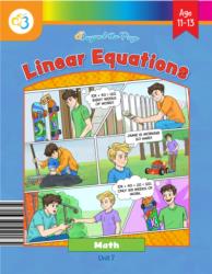
Students set up and solve linear equations that model real-world situations with a fixed fee plus a per-unit rate (e.g., 25 + 15x = 130; 18x + 20 = 146; 40 + 0.30x = 94). Students form equations for comparing two linear offers and solve for when the values are equal (e.g., 25 + 7x = 10 + 8x and other 'equal earnings' problems). The comic-strip activity and several word problems require students to define a variable, write a linear equation from a description, and solve for the unknown.

Students identify slope (m) and y-intercept (b) and use them to graph lines (Activity 5 shows y = 2x + 3 with points (0,3), (1,5), (2,7) and directions to use rise/run). Students convert equations into slope-intercept form and compare slopes and intercepts to classify systems (Activity 6 asks students to rewrite equations as y = mx + b and decide one/none/infinite solutions). Students substitute given points into equations to verify solutions (several examples substitute (1,3) or (1,-2) to show a point satisfies both equations).

Students compute slope from two points and write equations in slope-intercept form (examples show calculating slope with (y2-y1)/(x2-x1) and finding b, e.g., Line A: (0,0),(2,4) → y=2x and Line B: (1,6),(3,2) → y=-2x+8). Multiple activity pages ask students to plot two points, draw the line, and read or estimate intersection points from graphs (e.g., graphing y=2x and y=3x and noting slopes and the origin). Tasks repeatedly require students to find the equation of a line from two points and to identify slope and y-intercept when solving systems by substitution or elimination.

Students are asked to define variables and write linear equations in slope-intercept form (e.g., Total Cost = Rate × Quantity + Fixed Amount; y = mx + b). Students create functions from verbal descriptions (e.g., Sparkle Clean: y = 20x + 50 and Shiny Solutions: y = 30x; CinemaNow: y = 2x + 15 and StreamMore: y = 5x). Students solve those linear functions (by substitution) to find break-even points as coordinate pairs (e.g., (5,150) and (5,25)) and state which option is cheaper before and after the break-even point.

Students compute slope from two points (several problems ask for the slope through given point pairs and students find m = (y2−y1)/(x2−x1)). Students write equations of lines from two points and from given forms (tasks asking to find each line's equation from two points and to graph y = 2x − 1 or y = −3x + 2, with answers listing slope and y-intercept). Students model real situations with linear expressions (word problems such as "Jamie earns $12 per hour plus a $50 bonus" and gym/class or ticket problems require writing and solving equations like 12h + 50 = 122).

Students write linear cost equations from real descriptions (e.g., Housing: C = 1200m and C = 1500 + 1050m) and from provided numeric data (Transportation: C = 225 + 0.60x and C = 1.25x). Students graph those equations (housing, transportation, streaming, meal plans, phone plans), read y-intercepts and slopes from graphs (Meal Plans: identify fixed cost $100 and weekly rates $80 and $50), and complete tables of values (Phone Plans table and housing cost table). Students solve pairs of linear equations to find break-even points (set equations equal and solve by algebra, substitution, and elimination) and answer reflection prompts that interpret the rate of change and initial cost in context.

Students practice identifying independent and dependent variables, labeling axes, and distinguishing linear from non‑linear relationships. They choose or draw best‑fit lines (including selecting the best line from multiple options and drawing their own) and extend those lines to make predictions from a graph. Activities ask students to read trends from scatterplots, compare variability around a line, and use the line to estimate values (interpolation and extrapolation).

Students plot ordered pairs from tables onto scatterplots, choose axes and scales, and draw a best‑fit line (steps explicitly list labeling axes, finding range, choosing scale, plotting points, and drawing a best‑fit line). The activities ask students to decide whether a relationship is linear, describe positive or negative linear trends, and make numerical predictions from the graph or table (e.g., predicting a grade at 8 hours and noting "each additional hour studied corresponds to approximately a 10% increase"). Multiple student pages require reading data from tables and graphs and answering interpretation questions about trends, clusters, outliers, and predictions.

Students are shown how to find slope from two points using the slope formula and apply it to get an equation (example uses points (0,5) and (1,6) to produce y = x + 5). Multiple student activity pages require students to read scatterplots, identify the slope and y-intercept, write the equation in y = mx + b form, and choose matching equations for best-fit lines. The Bird Migration and other problem pages ask students to calculate the rate of change using two points, form the linear model, interpret slope and intercept in words, and use the model to make predictions.

Students are asked to write or choose linear equations that model plotted data (e.g., Question 13 asks students to select between y = 2x + 4 and y = 4x + 0, and Question 14 asks students to write an equation from a scatterplot). Multiple activities provide paired (x,y) data tables and blank graphs (e.g., Hours of Video Games vs. Homework, Missing Assignments vs. Test Score) where students plot points, assess linearity, and make numerical predictions (answers include specific linear equations such as y = 4x + 2, y = −8x + 40). The Parent Plan explicitly describes using the equation of a linear model to solve problems and interpreting slope and intercept with a contextual example (1.5 cm/hr).

Students collect paired numerical data, label axes, choose scales, and plot each (x,y) point on a scatterplot. Students are prompted to informally fit a straight line (line of best fit) and to analyze the scatterplot by identifying positive/negative association, clusters, and outliers. Students are asked to interpret what the observed trend means in the real-world context (e.g., as jumping jacks increase, heart rate increases). The Parent Plan explicitly expects students to use the equation of a linear model to solve problems and to interpret slope and intercept.

Students compute unit rates from two quantities (Activity 1 runner and cyclist problems) and compare unit rates to decide which is greater. Students write and match equations such as y = 6x, y = 4x, y = x + 2, and y = x + 6 to tables (Activity 2) and are asked to write an equation, create a table, and graph a proportional relationship (Activity 3 Create & Graph). Students graph y = 6x, label points including (0,0) and (1,6), and answer what those points represent, and several items ask for the constant of proportionality and interpretation of points like (0,6).

Students read tables and graphs and write matching linear equations (Activity 2 asks students to determine proportionality, find the unit rate, write y = kx from a table and graph, and interpret (0,0)). Activity 3 has students compute slope from two points, identify the y-intercept, and write equations in the form y = mx + b, including a real-world delivery-service scenario where they write y = 18x + 12 and identify slope and initial value. Activity 4 has students graph given linear equations from descriptions (phone plans and job offers), compare rates of change, and compute and compare costs at specific x-values, with answer keys interpreting slope as rate and the intercept as a starting fee.

Students write linear equations from contextual descriptions (e.g., C = 11t + 4 for movie tickets) and compute costs from those equations. Multiple problems ask students to find unit rates and constants of proportionality from tables and graphs (Unit 2 table, runner problems, question 19 and 34). Students compute slopes and y-intercepts from given points and equations (questions 35, 36, 37) and one answer explicitly interprets slope and intercept for y = 4x in context (answer key for question 20).

Students write linear functions from verbal situations and identify slope and initial value (Activity 4: write y = 18h for earnings; bike rental y = 12x + 10 with y-intercept = 10). Students compute slope/rate of change from two points and interpret it in context (Activity 3: find slope from (2,1) and (6,9) and explain its meaning; compare Function A and Function B given by points to determine which has greater rate of change). Students find and interpret intercepts from equations, tables, and graphs (Activity 2: find the y-intercept of y = 3x + 4, find the x-intercept from a table, identify intercepts from a graph and from 2x + 3y = 12; taxi scenario asks which intercept represents starting cost).

Students write linear equations to model real situations (e.g., 25 + 15m = 100, 6 + 2m = 34) and solve for unknowns in Activity 4. Students compute slope from two given points and graph lines given in slope-intercept form (y = x - 3, y = -2x + 1) in Activity 2. Students practice solving linear equations and systems (graphing intersections, substitution, elimination) across Activities 1–3, reinforcing connections between equations, graphs, and contextual problems.

The Parent Plan explicitly says students will informally fit a straight line to scatterplots and "use the equation of a linear model to solve problems..., interpreting the slope and intercept," and gives an example interpreting a slope. Activity 3 (Scatterplots & Linear Models) has student tasks that ask students to identify correlation, interpret relationships, and answer "What does it mean if most data points are close to the line of best fit?". The resources list includes a web link titled "Write an Equation for a Line of Best Fit," indicating instruction related to forming linear models.

Students write linear functions from verbal descriptions (Problem 8: "You earn $10 per hour. Write a function...") and set up linear equations from context (Problem 35: tutor charges $18/hour plus $30 fee). Students determine rate of change from two points (Problem 5 asks for slope through (2,4) and (16,12)) and read intercepts from equations, tables, and graphs (Problem 3 finds the y-intercept of y=3x+4; Problem 4 asks for the x-intercept from a table; Problem 6 has students graph y=2x-4 and Problem 9 asks for both intercepts).