


Eighth Grade - MATH
3: Math
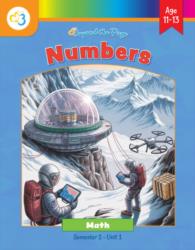
Unit 1: Numbers
Lesson 7
Arctic Marine Research
Students work with explicit exponential functions (N = 2^t and 3^t) in Phase 3, calculating populations after given intervals and comparing growth rates. Students also compute doubling via 2^10 for DNA replication, giving concrete non-linear function examples they evaluate numerically. The activities ask students to classify numbers involving square roots (√2, √50) and to convert decimals to fractions, which provides additional practice distinguishing types of functions/expressions.
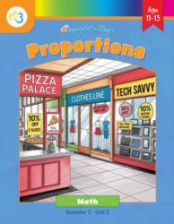
Unit 2: Proportions
Lesson 3
Constant Rate
Students repeatedly work with equations in the form y = kx and practice rewriting and identifying k (Activities 4 and 5). Students identify whether lines that pass through the origin represent proportional relationships and pick points on graphs to compute k (Activity 3). Students sort and classify equations, including non-linear examples (y = 3x^2, y = 3/x) and mark equations with extra terms (y = 2x + 3) as not proportional (Activities 4 and 5).
Lesson 4
Graphing Proportions
Students repeatedly write and use equations of the form y = kx and identify k as the unit rate (e.g., Jim's earnings y = 12x, examples y = 4x, y = 5x, y = 2x). Students plot tables and equations, draw straight lines through the origin, and check whether a graph is a straight line through (0,0) to decide proportionality. Students also test tables for equivalent ratios and identify non-proportional examples (ice cream prices, Bottle B, the cell phone data example, and the y = 60/x example) by showing the ratios or graphs are not constant or not straight through the origin.
Lesson 5
Proportional Relationship Equations
Students write and use equations in the form y = kx and t = p × n to model proportional relationships and complete tables of values (e.g., t = 12n for movie tickets, t = 15n for pizza). Students identify that a proportional relationship graphs as a straight line through the origin and practice finding the constant of proportionality and unit rate from tables and graphs. Students complete items that ask them to decide whether given scenarios or equations represent proportional (linear through origin) relationships and choose among equations such as y = 3x + 5, y = 7x, and y = 4x - 2 on a quiz item.
Lesson 6
Taxes, Tips, and Commissions
Students set up and solve percent-based equations such as 0.012 × V = 2400 and 1.08 × x = 212 when working backward to find property value or pre-tax price. Students use formulas written as linear multiplicative relationships (Commission = Sales Amount × Commission Rate; Gratuity = Tip Percentage × Original Bill) and solve problems that move forward and backward. Students practice solving equations and applying proportional reasoning in many problems (sales tax, income tax, tips, commissions).
Lesson 9
Unit 2 Test
Students work with and write equations in the form y = kx (e.g., y = (2/7)x, y = 4x, y = 5x, y = 9x) and identify the constant of proportionality from tables and equations. Students graph equations like y = 4x and analyze graphs labeled with points such as (0,0), (1,r), (8,36) to decide whether relationships are proportional. Several problems ask students to determine whether pairs of ratios or tables are proportional and to explain why (including circling "proportional" or "not proportional").
Final Project
Lemonade Stand
Students create tables and graph relationships between quantities (number of lemons, total cost; cups, tablespoons) and are asked to label axes, plot points, and draw lines. They are explicitly prompted to write equations in the form y = kx for the recipe scaling and to identify proportional relationships that produce straight lines through the origin. Students are also asked to compare slopes (steepness) of plotted lines and relate steepness to unit price.
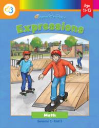
Unit 3: Expressions
Lesson 2
Rewriting Expressions
Students write and use expressions of the form Total Cost = Fixed Cost + (Variable Cost × # of Items), e.g., Total Cost = 25 + 3r, and set up and solve equations from those forms. Students rewrite selling-price and tax/discount relationships as one-step multiplicative expressions such as Selling Price = Wholesale Price + (Wholesale Price × Markup Rate) and Total Price = Original Price × (1 + Sales Tax Rate). Students solve for unknowns in these linear equations (for example, solving 58 = 25 + 3r or rearranging 31.50 = P(1.05) to find P).
Lesson 4
Graphing Proportions
Students make tables and plot points for equations such as y = 3x, y = 2x, y = 1/2x, and y = 4x and connect them to form straight lines that pass through the origin. Students compute the constant k by dividing y by x and interpret k as the unit rate (how much y changes when x increases by 1). Students analyze provided graphs (including a nonlinear curve in Graph B and a line that does not pass through the origin) and explain why those relationships are not proportional.
Lesson 5
More Graphing Proportions
Students repeatedly write and graph equations in the form y = mx (e.g., y = 4x, y = 2x, y = 2.5x, y = -3x) and plot points that produce straight lines through the origin. Students calculate slope from two points and from tables using m = (y2 - y1)/(x2 - x1), identify the slope m as the unit rate, and compare steepness of lines to determine greater rates. The lesson also contains the explicit statement that "if an equation is written in the form y = mx + b, the slope is always m."
Lesson 6
Intercepts
Students practice with equations in slope-intercept form (for example y = 5x + 10, y = -2x + 6, y = 3x - 9) and plot the corresponding lines by finding x- and y-intercepts. The materials instruct students to find intercepts algebraically by setting y = 0 or x = 0 and to plot those ordered pairs and draw a straight line through them. The Parent Plan and Things to Know sections state and ask students to derive y = mx and y = mx + b for lines through the origin and with a vertical intercept, and students graph lines using those forms.
Lesson 8
y = mx + b
Students repeatedly work with equations in the form y = mx + b: they derive y = mx for lines through the origin and y = mx + b for general lines, identify m as slope and b as the y-intercept, and graph many examples in activities (Comparing Graphs, Y-Intercept role, Negative and Zero Slopes, Graphing Equations). Students use tables and two-point calculations to find m and b, convert standard-form equations into y = mx + b, and plot lines to observe that these equations produce straight-line graphs and parallel lines when slopes match.
Lesson 9
Unit 3 Test
Students convert and rewrite equations into slope-intercept form (y = mx + b) and identify slope and y-intercept in multiple tasks (e.g., identify slope and y-intercept of y = -4x + 2; write an equation with slope 3 and y-intercept -5). Students find slope from a graph, a table, or two points (m = change in y/change in x) and use slope and intercepts to graph lines, extend lines, and write equations from plotted points. Several problems ask students to determine whether relationships are proportional or non-proportional and to write linear equations from context (e.g., earnings problems with fixed start-up fees and per-unit rates).
Final Project
Planes, Trains, and Automobiles
Students write equations in the form y = mx for distance vs. time (car: y = 60x; train: y = 80x; plane: y = 400x) and fill tables using those equations. Students plot those equations on a graph, compute rise/run, and answer questions about which lines are linear and proportional. In the cost activities, students write and use y = mx + b cost equations (e.g., y = 0.15x + 31.50), graph the lines, identify slopes (cost per mile) and y-intercepts (fixed starting costs), and solve for break-even points by equating linear equations.

Unit 5: Functions
Lesson 1
What Is a Function?
Students write and evaluate linear equations such as y = 2x + 6, y = 2x + 1, y = 3x - 4 and use them to fill input/output tables and plot points. Students plot those points and connect them to see that the points for these rules fall on a straight line and observe constant rate of change (e.g., y increases by 2 when x increases by 1). Students also work with non-linear rules like y = x^2 - 2 and other quadratic examples, compute outputs for given x-values, and plot those points to see a parabolic curve. Students use the Vertical Line Test on graphs (including a circle) to decide whether a graph represents a function.
Lesson 2
Linear and Nonlinear
The Parent Plan Skills section explicitly states the standard language, including interpreting y = mx + b and giving the nonexample A = s^2. Activity 2 has students work with the linear equation y = 2x + 4: they plug in x-values, compute y, calculate the constant rate of change, and view the plotted straight line with slope and y-intercept labeled. Multiple student activity pages require completing tables and graphing specific equations (y = x + 1, y = x - 4, y = 2x + 3) and identifying whether equations like y = x^2 and y = x^3 - x are nonlinear using their non-constant rate of change and plotted curves.
Lesson 3
Understanding Functions
Students are asked to tell whether a graph is straight or curved and to match straight-line graphs to constant-rate scenarios (e.g., Graph B: Constant Increase, earning the same amount of money every hour). In Activity 2 students compute positions from constant rates (Sylvia the Sloth, Timmy the Turtle, Bella the Balloon) and plot points that produce straight-line segments. The lesson explicitly asks and reviews how to tell if a relationship is linear (a straight line means the relationship is constant) versus nonlinear (a curve means the rate is changing).
Lesson 4
Intercepts
Students work with the slope-intercept form y = 2x + 3 and set x = 0 or y = 0 to find intercepts, showing use of an equation of the form y = mx + b. Students plot and identify intercepts on multiple straight-line graphs and find intercepts from tables and equations, reinforcing that these equations correspond to straight lines. Activities ask students to find intercepts for lines given in both standard form and slope-intercept form, and practice writing intercept coordinate pairs for those straight-line graphs.
Lesson 5
Slope
Students are introduced to slope-intercept form y = mx + b and told that m is the slope and b is the y-intercept. Students practice rewriting equations into y = mx + b (e.g., 4x + 2y = -8 → y = -2x - 4) and identify m and b from several example equations. Students plot points, connect them with straight lines, and use the slope formula m = (y2 - y1)/(x2 - x1) to find the slope between points, reinforcing that these equations describe straight lines. Multiple activities require students to find slope from graphs, tables, points, and equations, and to label slopes as positive, negative, zero, or undefined.
Lesson 6
Slope-Intercept Form
Students repeatedly work with the equation y = mx + b: the Things to Know section defines y=mx+b and labels m as slope and b as y-intercept, and multiple activities (Graph to Equation, Equation to Graph, Table to Equation, Simplify and Graph, Slope from Two Points) have students compute m and b and write equations such as y = 2x + 2. Students plot points and draw straight lines from those equations (e.g., using (0,2) and (3,8) to get y=2x+2) and convert standard-form equations into y=mx+b to identify slope and intercept for graphing. The opening narrative (Ellie's trips) and repeated graphing tasks require students to recognize that these equations correspond to straight-line graphs and to move between graph, table, point, and equation representations.
Lesson 7
Creating Functions
The lesson repeatedly presents the form y = mx + b and translates it into output = slope × input + starting value, telling students to rename y and x to match contexts (e.g., A = 6c + 12). Students practice finding slope and y-intercept from stories, tables, and straight-line graphs using the slope formula and then write function rules (several activities and examples show line graphs and tables that yield linear equations). Classroom activities require students to interpret points on a line, calculate m and b, and write linear functions from data and graphs.
Lesson 8
Comparing Functions
Students work with multiple equations in slope-intercept form (e.g., y = -3x + 100, H = 4x + 10, y = -10x + 50, d = 3t + 2) and are instructed that the y-intercept is b and the slope is m. Students calculate slope using the slope formula from graphs (example using points (0,0) and (30,2)) and from tables (Taylor's account, plant growth tables) and compare rates of change. Several activities require interpreting straight-line graphs and matching their slopes and intercepts to equations or verbal descriptions (e.g., walking pace, water-filling, bike race).
Lesson 9
Unit 5 Test
The Parent Plan Skills explicitly states interpreting the equation y = mx + b as defining a linear function and gives a non‑linear example (A = s^2). Multiple student tasks require finding slopes and y‑intercepts (e.g., "Find the y‑intercept of y = 2x + 3", "Graph y = 3x - 1"), creating equations from a given slope and y‑intercept, and interpreting slope as rate of change in context (earnings, distance/time). Several problems ask students to identify nonlinear equations (multiple choice selecting y = x^2) and to use the vertical line test or recognize curved graphs to label functions as nonlinear, and one activity explicitly has students complete a table for y = x^2 - 2 and mark it Nonlinear.
Lesson 10
Final Project
Students are asked to identify slope and y-intercept from equations (e.g., "What is the slope and y-intercept of y = -2x + 5?") and to classify equations as linear or nonlinear (e.g., "Is y = x^2 + 3 a linear equation?"). Students create blue cards that require writing equations from stories and matching equations to graphs, and green/yellow cards require writing equations from tables and real-world descriptions. The parent-plan skills explicitly state that students will "Interpret the equation y = mx + b as defining a linear function" and give examples of non-linear functions such as A = s^2.
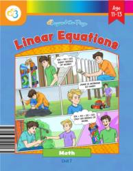
Unit 7: Linear Equations
Lesson 5
Intersection and Graphing
Students are explicitly asked to work with equations in the form y = mx + b and are told "Every equation in the form y=mx+b can be graphed as a straight line." Students identify m as slope and b as y-intercept, graph lines (e.g., y = 2x + 3), plot labeled points such as (0,3), (1,5), (2,7), and use slope-intercept form to compare slopes and intercepts to determine intersection behavior. Students convert standard-form equations to slope-intercept form (e.g., 4x−2y=8 → y=2x−4) and use substitution to verify that points satisfy linear equations.
Lesson 6
Substitution and Elimination
Students rewrite equations into slope-intercept form (y = mx + b) and graph those equations to find intersections, as shown in the instructions to put equations in slope-intercept form and the many graphing activities. The Linear Equation Forms table explicitly presents slope-intercept form y = mx + b and standard form Ax + By = C, and students practice plotting linear equations such as y = 3x, y = 2x, and y = -x + 1. Students also use Desmos to enter equations like y = 2x + 3 and observe the resulting straight-line graphs, reinforcing the connection between y = mx + b and a line.
Lesson 7
The Point of It All
Students find slopes from two points and write equations in slope-intercept form (y = mx + b) in multiple activities (e.g., sections asking "Find and write the equation of Line A/Line B" and the Parent Plan explicitly: write the equation of each line in slope–intercept form). Students graph those equations (examples throughout show y = 2x, y = -x + 6, y = 4x - 2, etc.) and draw straight lines through plotted points to estimate and identify intersections. The answer keys and worked examples set up equations as y = mx + b and use those equations to produce and interpret straight-line graphs and intersection points.
Lesson 8
Linear Algebra In the Wild
Students write and use equations in slope-intercept form (for example y = 20x + 50 and y = 30x, y = 2x + 15 and y = 5x) to model cost situations and find break-even points. Students solve these equations and systems (substitution/elimination) to find intersection points such as (5, 150) or (5, 25). Student activity pages ask students to write functions in the form y = mx + b (examples like y = 10 + 2.5x and y = 10 + 3.2x) and to create graphs to "see a picture of the solution."
Lesson 9
Unit 7 Test
Students are asked to graph equations given in slope-intercept form (for example, "Graph y = 2x - 1") and to find slopes from pairs of points (several problems ask for slope through given points). Multiple problems require writing line equations from two points and interpreting intersections (e.g., systems like y = -x + 4 and y = x - 2, and identifying parallel lines such as y = 3x + 1 and y = 3x - 5). The skills list and activities direct students to identify slope and y-intercept and to interpret points of intersection as solutions to systems.
Final Project
Getting Ready for College
Students write cost equations in slope-intercept form (for example C = 1200m and C = 1500 + 1050m for housing, C = 225 + 0.60x and C = 1.25x for transportation, C = 5 + 1.5h and C = 20 for streaming, and y = 5x + 20 for phone plans). Students graph these equations on coordinate grids, label the lines, identify y-intercepts and slopes (e.g., meal plan y-intercept and weekly slope), and interpret intersections as break-even points. Several answer keys and parent notes explicitly have students solve 2-line systems and reason that identical linear equations represent the same line.

Unit 8: Data
Lesson 2
Scatterplots
Students identify linear relationships by recognizing when scatterplot points form a straight-line pattern and label graphs as Linear or Non-Linear. Students draw or choose best-fit straight lines through data, judge whether about half the points lie above and below the line, and use those lines to make predictions. Students practice distinguishing linear (straight-line) patterns from curved or other non-linear patterns across multiple activities and examples.
Lesson 3
Constructing a Scatter Plot
Students repeatedly plot bivariate data and are asked to decide whether "there is a linear relationship" and to "draw a best fit line (if needed)." Multiple activities ask students to identify positive or negative associations, linear association, and nonlinear association (e.g., questions: "Is there a linear relationship on your scatterplot? How do you know?"). Several answer keys label particular datasets as "linear" or "nonlinear" and ask students to make predictions by extending a straight-line trend.
Lesson 4
Linear Models
Students repeatedly write and read equations in the form y = mx + b: activities ask them to identify slope and y‑intercept from lines on scatterplots, write equations for lines (Parts 1 and 2), draw or match best‑fit lines to equations, and substitute values to make predictions (ice cream, plant growth, tickets, etc.). The lesson explicitly labels these as linear models and directs students to interpret slope as change in y per unit change in x and the y‑intercept as the starting value. Several student pages require plotting points, drawing a best‑fit line, calculating m using two points, and forming the equation in y = mx + b format.
Lesson 6
Unit 8 Test
Students repeatedly classify relationships as linear or nonlinear on scatterplots (multiple questions ask "Linear or Nonlinear?" and the answer key labels relationships as linear). Students write and choose linear equations in slope-intercept form (examples in questions and answers include y = 4x + 2, y = 4x + 0, y = -8x + 40, and a choice between y = 2x + 4 and y = 4x + 0). The skills and parent plan explicitly tell students to use equations of linear models to solve contextual problems and to interpret slope and intercept in context.
Final Project
Collecting and Organizing Data
Students plot bivariate numerical data on scatterplots, label axes, choose scales, and are instructed to "draw a line that best fits the overall shape of the data" (Part 4 scatterplot instructions). The activities ask students to analyze patterns and identify positive, negative, or no correlation and to judge whether points form a linear association (Part 4 and Part 5 analysis prompts). The Parent Plan Skills explicitly state that students should "informally fit a straight line, and informally assess the model fit by judging the closeness of the data points to the line," and they mention using the equation of a linear model and interpreting slope and intercept.
Unit 9: Semester Exams
Lesson 2
Proportions Review
Students graph and label linear equations such as y = 6x, plot points like (0,0), (1,6), and draw the straight line through them. Students match tables to equations that include forms y = 10x, y = 3x, y = x + 2, and y = x + 6 and decide whether each relationship is proportional. Students respond to true/false prompts about proportional graphs, the form y = mx + b, identify the constant of proportionality (slope), and interpret points such as (0,0) and (0,6).
Lesson 3
Expressions Review
Students write equations in the form y = mx + b (Activity 3, Activity 4) and find slopes and y-intercepts from points, tables, graphs, and equations. Students graph linear equations and compare their steepness, recognizing that the plotted relationships form straight lines (Activities 2, 3, and 4). Students interpret slope as a unit rate and the y-intercept as an initial value in real-world contexts (answer keys and real-world problems such as delivery fee and babysitting pay).
Lesson 5
Semester Exam
Students are asked to graph and describe y = 4x (problem 20) and the answer key explains the slope is 4 and the line passes through the origin, representing a constant rate of change. Students identify slope and intercept for y = 3x + 8 (problem 36) and plot a line through (0,0) and (4,-8) asking for slope and equation (problem 37). Multiple items ask students to determine slopes and compare rates of change from points or graphs (problems 31, 35, and 19), providing practice interpreting m and recognizing linear behavior on the coordinate plane.
Lesson 6
Functions Review
Students identify slope and y-intercept from equations written in slope-intercept form (e.g., tasks with y = -1.25x + 5, y = 3x + 4, and 2x + 3y = 12) and graph lines (e.g., graph y = 3x - 2 and a plotted line through (-1,-3),(1,1),(3,5)). Students write linear functions from contexts (y = 18h, y = 12x + 10) and explain the meaning of m and b in real situations. Students are asked to distinguish linear from nonlinear equations (selecting y = x^2 + 3 as nonlinear) and to explain how a graph or an algebraic form (squared variable) indicates a nonlinear (curved) function.
Lesson 8
Linear Equations Review
Students practice graphing equations in slope-intercept form (Activity 2 asks them to graph y = x - 3 and y = -2x + 1) and compute slope from two points (Activity 2, Part B). They work with linear equations in multiple representations (equations, graphs, tables, and word problems) and model real-life linear relationships by writing and solving linear equations and systems (Activity 4). Several activities require solving for y and plotting lines, which shows students producing straight-line graphs from linear equations.
Lesson 9
Data Review
Students analyze scatterplots, identify positive/negative/no correlation, and interpret what a line of best fit indicates about a linear trend (Activity 3). The Parent Plan lists skills that include informally fitting a straight line to scatterplot data and using the equation of a linear model to interpret slope and intercept. The answer key explicitly states that points close to the line of best fit mean the data follows a linear trend, showing attention to linear association.
Lesson 10
Semester Exam
Students are asked to identify which equation is nonlinear (question 1 with answer B: y = x^2 + 3) and to explain how to tell from a graph whether a function is nonlinear (question 2; answer: the graph is curved or not a straight line). Students find the y-intercept of y = 3x + 4 and graph linear equations such as y = 2x - 4, and they write a linear earnings function y = 10x. The answer key language explicitly connects linearity to a straight line and constant rate of change (question 9b answer).